The residue gap and the chemistry
Rudolf's formula turns temporary gas uptake into a prediction of lasting cyanide residue. The uptake experiment didn't measure chemical binding. A model that calculates capture and escape separately can reproduce the size of the residue gap under the assumptions below. The section on formation examines what Rudolf’s proposed chemistry establishes about lasting residue.
| Comparison | Morgue 1 R3 | Delousing R12 | Delousing R13 |
|---|---|---|---|
| Reported assays | 6.7 initially Below detection on retest | 2,900 | 3,000 |
| Rudolf's lower bound, applied to each comparator | 2,442–2,526 | 2,900 | 3,000 |
| Range across the seven conditional variants | 8.18–551.93 | 2,884–5,787 | 3,053–6,127 |
The initial R3-to-R12 ratio is 1 to 433. Rudolf's corrected lower bound is about 1 to 1.19, roughly 364 times that initial ratio. The seven conditional variants give paired ratios from 1:352 through 1:10.5. All seven give a smaller gap than the initial assays' 1:433; none reproduces that ratio. Their spread shows how much the assumed capture law matters.
The last row spans seven alternative assumptions, not a confidence interval or a validated reconstruction. Every variant uses 400 daily chamber exposures and 400 six-hour delousing treatments spaced across 270 days. The model assumes the same basic material response in both room types. Five powers come from separate fits to aqueous experiments and are used beyond their measured concentration range; their applicability to these walls is unresolved. The complete paired results appear below. R3's later retest was below detection. These selected specimens aren't room averages.
Rudolf's formation model doesn't establish his residue bound
Rudolf's chemistry allows cyanide to accumulate and form Prussian blue. It doesn't establish how much must remain in the sampled wall. The high delousing residues are real. To turn their contrast with Morgue 1 into an exclusion of homicidal gassing, Rudolf needs a supported limit on how far the two walls' lasting, recoverable residues could differ. A temporary uptake ratio doesn't supply that limit. His account of later reactions has to supply the missing connection.
He proposes storage followed by reaction
Rudolf's argument goes beyond immediate pigment formation during contact with the gas. In his account, alkaline masonry converts hydrogen cyanide into soluble cyanide. Cyanide can remain available while it reacts slowly with iron compounds. Iron(II) cyanide can accumulate and later form Iron Blue near the zone where carbonation has lowered the pH. Carbonation is the reaction of carbon dioxide with alkaline masonry. Rudolf gives days or weeks for the alkaline period in lime mortar and months or years in cement mortar and concrete. He treats the longer period as an opportunity to retain cyanide and give it time to react, not simply as a delay that defeats formation. Rudolf 2020, page 222 · Page 223.
He also supplies a reason why some reaction could continue despite an unfavorable equilibrium. On page 196, note 227, he argues that reduction of iron(III) cyanide to iron(II) cyanide removes the first product from the equilibrium and allows further formation. He describes reactions at the solid surface and the reactivity of freshly precipitated iron hydroxide. This is a proposed chemical mechanism. Dismissing it as a statement about where a reaction happens would leave his actual argument unanswered. Page 196 and note 227.
The unanswered question is how much cyanide this route captures and preserves in each wall. A soluble precursor can react, move with water, or escape after conversion back to hydrogen cyanide. Rudolf himself invokes moisture-driven migration of soluble cyanide salts when discussing wall profiles. That is part of his explanation, not a measurement of how much left a sampled layer. Rudolf 2003, page 263. Establishing one possible route doesn't establish its share of the inventory. Rudolf's numerical comparison needs that share, or a defensible bound on it, under the relevant material and exposure conditions.
Equilibrium constants don't give a formation rate
Meeussen's 1992 thesis gives log K = 43.9 for formation of the iron(III) cyanide complex from Fe³⁺ and six CN⁻ ions. A separate table gives log K = 3.54 for dissolution of the iron hydroxide used in that calculation. Combining those specified reactions gives the following balanced relation, with water written explicitly. Meeussen's thesis, page 31 · Page 80.
Fe(OH)₃(s) + 3H⁺ + 6CN⁻ ⇌ Fe(CN)₆³⁻ + 3H₂O
log K = 3.54 + 43.9 = 47.44
This is a conditional equilibrium calculation, not a universal masonry constant. Page 31 uses a different hydroxide constant, 2.7, in its soil calculation. Neither number identifies the reactive iron phase in a particular sampled plaster. The 49.9 entry on that page already includes Fe³⁺ and an electron in forming iron(II) cyanide. Adding a separate iron-reduction constant to it would count that step twice.
Even the direction of the pH effect depends on what is held fixed. In the first relation, the dissolved product at equilibrium depends on H⁺ cubed and free CN⁻ to the sixth power. Those terms use activities, concentrations adjusted for interactions in the solution. At fixed free CN⁻, increasing pH decreases the calculated product. At fixed neutral dissolved HCN, acid-base equilibrium makes free CN⁻ increase as H⁺ falls. Substitution then reverses the pH dependence. A gas concentration, a free-ion concentration, and a total cyanide inventory aren't interchangeable inputs.
The powers in that equilibrium expression aren't measured reaction orders. They don't tell us how much product forms in minutes, days, or years. Nor does a small dissolved concentration cap the total solid that can accumulate when reactions remove dissolved products. Rudolf's proposed reduction step is precisely why that distinction matters. The constants alone can't put the two historical walls on opposite sides of a formation threshold.
Short gas contact doesn't settle the later chemistry
A shorter exposure can reduce uptake. It doesn't establish that all subsequent reaction stops when ventilation begins. Rudolf expressly relies on retained cyanide reacting later. His note 268 also says that very humid mortars and concretes have no sharp carbonation or pH boundary because of proton diffusion. An argument built around a single front arriving after all cyanide has escaped would contradict that qualification unless the relevant timing were established independently. Page 222, notes 267–268.
The building's construction dates don't establish the pH history of the sampled plaster, its retained cyanide, or its later reaction rate. No such history has been established here. It follows neither that Morgue 1 had to form substantial pigment nor that its cyanide necessarily disappeared before pigment could form. The unsupported claim in Rudolf's comparison is the required residue bound. Replacing it with an unsupported chronology wouldn't answer it.
Alkaline breakdown isn't proof that no pigment survives
Rudolf discusses alkaline decomposition on page 208 and gives about pH 10 as the point where removal of iron as hydroxide begins in the case he describes. On page 337 he says Iron Blue paint on fresh mortar would decompose and lose its color at least temporarily. These passages support the importance of chemical conditions. They don't establish instantaneous destruction of every crystal in every alkaline wall. Page 208 · Page 337.
Rudolf's numerical solubility argument also skips a necessary step. On page 208 he takes one quarter of the free ferric-ion concentration as the amount of pigment dissolved. Four is the correct count of iron atoms outside the three iron-cyanide groups in his formula. But free ferric ions aren't the whole dissolved ferric component: iron can also occur in dissolved complexes with hydroxide and other substances. Rudolf acknowledges those forms on the same page. Their amounts still have to be included before free-ion concentration can be converted into total pigment solubility. His calculation doesn't establish the extraordinarily small total solubility he quotes. This defect supplies neither a corrected dissolution rate nor a prediction of how much pigment a historical wall lost. Rudolf 2020, page 208.
His page 209 gives two distinct defenses of stability. One concerns aged crystals formed slowly in roughly neutral, carbonated masonry. The other concerns freshly precipitated, pure Iron Blue formed without co-precipitating iron hydroxide, which he says remains stable further into the alkaline range. The second defense isn't restricted to an already aged crystal. Contact with existing solid hydroxide doesn't, by itself, prove that hydroxide co-precipitated with the pigment. Page 209.
The exact Ghosh equilibrium paper Rudolf cites for that second defense hasn't been obtained. The separate Ghosh transport paper doesn't settle its experimental conditions or its application to a wall. The defensible conclusion is narrower than either a universal stability claim or a universal destruction claim.
Meeussen and colleagues found a further reason to distinguish equilibrium from actual persistence. In their 1994 soil study, Prussian blue persisted decades after disposal even where their equilibrium calculation predicted dissolution. At the site they called alkaline, measured extract pH rose from 5.5 in the upper material to 7.2 deeper down. They considered slow dissolution, local buffering, and transport as explanations; their five-day extraction hadn't reached equilibrium. This wasn't a test of fresh cement at pH 12–13, and it doesn't supply a masonry lifetime. It does show why an equilibrium prediction alone can't establish prompt disappearance. Meeussen et al. 1994, page 790 · Page 791.
Loss of blue and loss of cyanide are different measurements
Alkaline breakdown can leave dissolved ferrocyanide, the iron(II) cyanide complex. Disappearance of the blue color therefore doesn't establish disappearance of all cyanide. Ware describes that distinction in discussing cyanotypes. Any claim about a later total-cyanide result also needs to account for what remained, what left the specimen, and what the assay recovered. Ware 2003, page 13.
Leaching experiments show that substantial loss is possible under their conditions. Markiewicz, Gubała, and Łabędź removed 82 to 91 percent of recoverable cyanide by flushing small, 0.5-gram plaster samples with a liter of water. Kamat, Lubelli, and Schlangen reported loss of more than 80 percent of an added ferrocyanide inhibitor from mortar in a ten-day tank test. The latter used a high initial loading and replenished leachant. Neither experiment measures loss from the intact historical wall, and neither result is a direct measure of the disappearance of its Prussian blue. The dossier's discussion of retention sets out these conditions; the Kamat paper gives the mortar experiment.
Lower formation and later loss can both contribute to a low result. They can also be investigated separately. Neither has been established here as the quantitative explanation of the historical residue gap, and the same loss can't be counted twice. The real, persistent delousing residues remain evidence that large amounts can survive in some walls.
Rudolf's mortar tests measured retained cyanide
Rudolf's cement-mortar specimens R27 and R28 retained 109 and 94 milligrams of cyanide per kilogram after the reported exposure and storage. These are positive measurements of retained cyanide. They aren't measurements of a specified Prussian-blue fraction. Failure to identify the pigment can't be rewritten as proof that it was absent. Rudolf 2020, page 327 · Page 328.
The recipes also differ: R27 contains lime and R28 contains chalk, and the preparation table describes both as moist. Their small final-residue difference therefore isn't a controlled measurement of moisture alone. It remains a result any account of those particular specimens must explain. It doesn't supply a universal wet-to-dry correction for historical walls.
A low true total cyanide inventory limits the cyanide that can be bound in pigment, when both are expressed on the same cyanide-mass basis. Applying that limit to an assay requires adequate recovery and uncertainty estimates. A total measurement doesn't identify the pigment fraction. The distinction also matters for R3, initially reported at 6.7 mg/kg and later as not detected. Neither treating that later result as zero nor treating the example's 8.18 mg/kg as validated agreement is justified by an unspecified effective detection limit in that matrix. The experimental limits remain part of the comparison.
The high delousing results still have to be explained
Sample R17 contained 13,500 milligrams per kilogram at a depth of 4 to 10 millimeters. The residue wasn't confined to a visible surface stain. Rudolf's low controls from walls added during conversion to hot-air disinfestation had a different exposure history. They aren't matched examples of original exposed delousing walls yielding little cyanide. Their low results can't be used to erase the high results from the original walls. Rudolf 2003, Table 19, page 254 · Page 263.
Bailer, as quoted by Rudolf, argued that trivalent iron and an alkaline environment impeded formation. Rudolf's reply discusses surfaces of corroded bricks as well as stained mortar and plaster. That exchange can't be settled by saying that his reply concerned brick while Morgue 1 was concrete. His broader retained-precursor and surface-reaction argument still needs the direct answer given above. Rudolf 2020, page 339.
The missing quantity is lasting, recoverable residue
It isn't mathematically wrong to multiply factors for successive stages when the connection between them is supported. The failure is to treat a temporary uptake comparison as if it fixed the ratio after storage, chemical conversion, escape, weathering, and assay recovery. Rudolf supplies reasons that pigment can form and persist. Those reasons don't establish the minimum residue his exclusion requires in the other wall.
The conserving calculation on this page demonstrates the consequences of its stated assumptions. Its aqueous reaction fit hasn't been established as the reaction law of historical masonry, and the alternative fits remain visible. The historical balance among capture, reaction, and loss hasn't been reconstructed. That limit doesn't rescue Rudolf's calculation. His claimed exclusion still needs the quantitative connection his uptake factors and proposed chemistry haven't established.
What the evidence supports
The residue evidence does not show an absence of cyanide exposure in the morgue ruins. The Kraków institute's procedure, chosen not to decompose Prussian blue and checked on a standard, recovered cyanide from thirteen of fourteen Krematorium II and III specimens, with individual determinations up to 640 micrograms per kilogram, and reported all eight of its designated dwelling controls as zero. Those controls had probably been fumigated once themselves. The same procedure gave up to 900 micrograms per kilogram in delousing samples, where Rudolf's separate total-cyanide assay found thousands of milligrams per kilogram; the two were not paired determinations on the same specimens. The repeated detections and the contrast with the controls support prior HCN exposure in the morgue material. They do not by themselves determine the number, duration or purpose of the exposures. The tables and page references are on the refutation page.
Exposure does not translate directly into the total inventories the delousing walls hold. Uptake, escape, precursor formation and lasting retention are distinct, condition-dependent processes. The experiments Rudolf reprints show both directions at once: well-dried cement mortar yielded 200 milligrams of recoverable hydrogen cyanide per square meter at the end of a 24-hour exposure and 80 after 22 hours of airing, while still-fresh concrete yielded 5,198 and still 1,926 after 90 hours, and Rudolf writes that the method cannot establish long-term binding. His own mortar test retained 109 and 94 milligrams of cyanide per kilogram after 71 days of dry storage with no visible blue, and he writes that drying "strongly hindered" and "probably blocked" the conversion. A retained-cyanide measurement does not identify the pigment fraction, and a positive cyanide result does not require a visible stain. The uptake and retention section and the mortar test carry the pages.
Ventilation limits the supply of gas to a wall. It does not itself stop the chemistry inside it, and Rudolf's own mechanism allows iron(II)-cyanide to accumulate in strongly alkaline masonry and react later. The model on this page keeps both. Calibrated to his mortar endpoint and run on his own two exposure branches, it can produce low morgue residue and high delousing residue on his 14.4-minute branch under stated assumptions, and it does not reproduce that pattern in any tested 72-minute case. The result depends on a capture law motivated by solution experiments, exchange times borrowed from other specimens, an assumed mobile capacity, an unverified relationship between the two materials, and assumed gas histories and treatment schedules. Within the model, low morgue residue and high delousing residue coexist even though mobile cyanide carries over between exposures and captured product is never destroyed. That is mathematical compatibility, not a validated reconstruction of these walls.
Alkalinity, carbon dioxide, washing and the church cases are constraints on any account, not multipliers that supply what the model lacks. Rudolf leaves the carbon-dioxide effect out of his calculation and says its influence is not known; the Kraków series with added carbon dioxide behaved differently from the series without it. Washing and airing reduced the fraction the Kraków procedure recovers in small laboratory pieces, which is a measurement of that fraction, not of pigment destruction in a wall. The technical report on the Untergriesbach church identifies calcium cyanide and dark polymer products and does not identify Prussian blue. The same authors' dry-weather comparison at Thundorf showed no notable damage. Wiesenfeld remains a single-fumigation case whose technical record has not been read. The church comparison and washing and weathering are treated on the refutation page.
Rudolf's expected minimum does not follow from any of this. His uptake ratio, his cement argument, his exposure calculation and their product do not bound the conversion, retention and material-transfer relationships that connect gas taken up to residue recovered decades later, and his own text keeps an unquantified exception for carbon dioxide and allows suppressed formation or later loss. His comparison has not established the necessity his conclusion requires. The measured gap is compatible with mechanisms his numerical bound does not establish or exclude. Saying that this is exactly what the historical exposures would leave would be more than the evidence supports; that sentence is not made here.
Gas taken up by a wall can leave again
Hydrogen cyanide, HCN, can enter moisture in a wall and later escape. A smaller share can react with iron to form ferrocyanide, an iron ion bound to six cyanide groups. Further reaction can form Prussian blue. A measurement of gas that escapes doesn't measure how much completed those reactions and remained in the sampled material.
Rudolf recognized the distinction. His footnote 410 on page 187 says the uptake test couldn't establish chemical binding because it measured only the HCN that evaporated. On page 283, he nevertheless uses an eightfold uptake factor in his prediction of iron-cyanide residue. His argument about damp cement requires a supported numerical link between those quantities. His formula and the source pages.
In the conditional model, both room types receive the same gas concentration during exposure. A long exposure maintains more cyanide inside the wall than a brief pulse. With a capture rate that rises roughly with the square of mobile cyanide, that difference produces a much larger difference in accumulated residue. Halving mobile cyanide reduces the instantaneous capture rate to about 23% in the law used here.
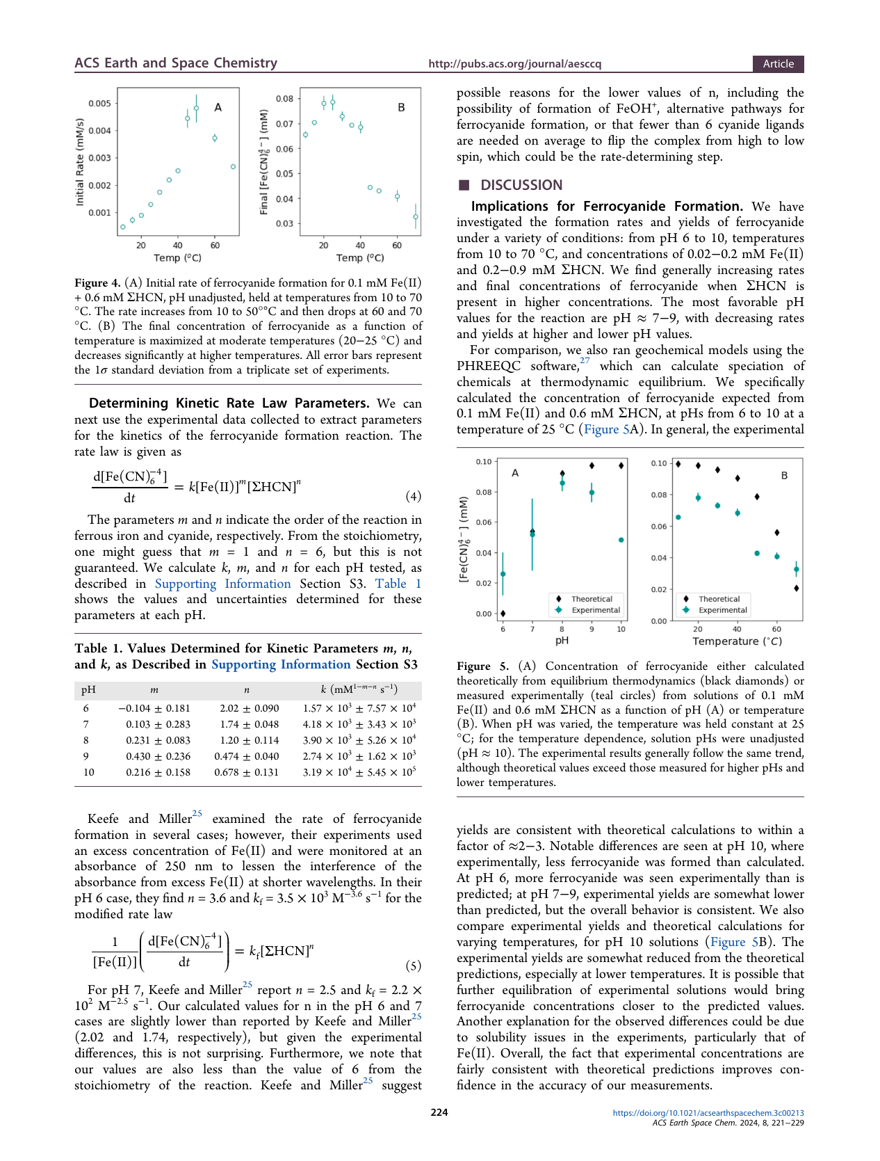
Todd, Wogan, and Catling measured concentration-dependent ferrocyanide formation in water. Their pH 6 results supply the near-quadratic example. Fresh cement can be strongly alkaline; these pages don’t establish that its reacting pore water followed the pH 6 solution experiment. The higher-pH fits give much higher chamber residues, as the seven-variant table below shows. Todd and colleagues didn’t measure permanent pigment formation in masonry. Applying that law to the mobile wall inventory is an explicit assumption. The measured reaction and its limits.
One laboratory result calibrates both comparisons
Rudolf's cement-mortar specimens R27 and R28 gave 109 and 94 mg CN/kg after exposure and storage. The model uses their mean, 101.5, adjusted to R3's total iron content as 115.34 mg/kg. For each assumed capture law, one coefficient is chosen to reproduce that laboratory endpoint. The same coefficient then calculates the short exposures and the delousing exposures.
| Capture law | Rate proportional to mobile cyanide raised to 2.10733. This is a separate fit to Todd's pH 6 raw data, transferred to a wall model. |
|---|---|
| Laboratory endpoint | 24.75 hours at 2% HCN by volume, at 11°C, followed by 71 days of storage. The total-cyanide result is treated as permanently retained product. The model keeps the same exchange law during storage, though the actual samples dried at room temperature. |
| Mobile inventory | 500 mg CN/kg at equilibrium with the laboratory reference gas. A Henry-law estimate gives 546 mg/kg if the material contains 0.03 liters of water per kilogram. That water content wasn't measured in R3. |
| Exchange with air | Two contributions with characteristic release times of 7.2 and 96 hours, derived from Rudolf's fit to another material's release curve. Both feed an assumed common reacting pool. |
| Chamber exposures | 400 daily rectangles, each 14.4 minutes at 10 g HCN/m³. This is Rudolf's shorter equivalent-contact branch, not a measured time of death or a recovered gas trace. |
| Delousing exposures | 400 six-hour rectangles at 10 g HCN/m³, starting every 16.2 hours within 270 days. The table below also tests daily treatments and a schedule with 130 double-treatment days. |
| Material transfer | R12 and R13 use 0.85 and 0.90 times the R3-normalized mobile capacity, capture throughput, and total iron capacity. This assumes these quantities scale together with total iron. |
The calculation keeps every remaining mobile inventory between exposures and continues capture during airing. Every scenario includes a final 71-day clean-air period. Captured product never disappears, and the iron inventory is finite. The selected example assumes reactive iron can be supplied fast enough for the capture law; it imposes no separate delivery-rate limit. No percentage for washing, weathering, demolition, or CO₂ is used to obtain the low result.
R27 and R28 are different specimens, not repeat measurements of one specimen. The 2020 preparation table gives different added-water conditions and prints lime for R27 but chalk for R28. Their average supplies a common calibration, but doesn't establish a unique material response. R3, R12, and R13 weren't used to fit the coefficient. The displayed combination was selected after reviewing the scenario grid, so its numerical agreement isn't an independent validation.
How our inputs differ from Rudolf's
Rudolf's later calculation already includes diffusion and repeated exposure. Our model adds an explicit calculation of capture competing with escape. It also makes different material assumptions, so the numerical disagreement can't be attributed to that added reaction step alone.
| Input | Rudolf | This example | Reason and limit |
|---|---|---|---|
| Gas concentration | 10 g/m³ in both room types. | The same concentration. | The low chamber result doesn't come from reducing the gas concentration. |
| Chamber contact | 14.4- and 72-minute equivalent exposures. | The shorter branch, 400 times at daily starts. | It is his own branch, but assumes introduction columns and nearly perfect ventilation. The choice favors low retention. |
| Delousing use | Six-hour and twelve-hour daily examples. His comparison says probably fewer than 400 treatments. | 400 six-hour treatments across 270 days. | This fits the calendar and improves the numerical match. It isn't a recovered treatment history. |
| Moisture and cement | An eightfold uptake factor and an assumed cement factor of two. | The same basic material response, scaled with total iron. | A common-material example doesn't establish equal behavior in the historical walls. His factors aren't direct measurements of their residue ratio either. |
| Chemical capture | Loading and material factors become a prediction of iron-cyanide residue. | A near-quadratic capture law competes with escape. | This makes the formation step explicit. The aqueous law, assumed water content and reactive iron supply still need to describe a compatible wall system. |
| Calibration | Laboratory tests and material comparisons support his argument. | The mean of R27/R28 sets one capture coefficient. | The coefficient isn't fitted to R3. Averaging different preparations and selecting the displayed scenario after comparison don't make its agreement an independent validation. |
Rudolf's eightfold factor has a source in the reported wet/dried lime-sandstone uptake comparison. He explicitly says that method couldn't establish long-term binding. The supported objection concerns his later prediction of residue, not the fact that moisture affects uptake. Uptake table, page 223 · Measurement limit, page 224 · Diffusion calculation, page 285 · Absolute loading, page 286 · Treatment counts and comparators, page 357.
If the model's mobile inventory is dissolved in the assumed 0.03 liters of water per kilogram, its final chamber cycle spans 1.96–4.21 millimolar and its final delousing cycle spans 41.93–74.70 millimolar. The calibration exposure peaks at 174.46 millimolar. Todd's experiments covered 0.2–0.9 millimolar. Millimolar means millimoles per liter. These are concentrations inferred from our assumptions, not measurements of wall water. They show that borrowing the measured reaction order also requires a substantial extrapolation in concentration. The experiment and its limits · Concentration calculation.
The spacing between treatments changes retention
The original near-match uses 400 daily delousing treatments and therefore needs about 400 days. It doesn't fit within a 270-day comparison period. Four hundred six-hour treatments can fit arithmetically into 270 days if some days contain two treatments, but the shorter gaps change the chemical result. Here six hours means the model's constant-concentration exposure, not a measured elapsed treatment time. An actual twelve-hour treatment with falling gas concentration doesn't establish that input.
| Assumed schedule | R12 | R13 |
|---|---|---|
| 400 daily treatments, about 400 days | 2,442 | 2,586 |
| 270 daily treatments, 270 days | 1,646 | 1,743 |
| 400 treatments at 16.2-hour intervals, 270 days | 2,884 | 3,053 |
| 400 treatments with 130 double-treatment days and 140 single-treatment days, 270 days | 2,920 | 3,091 |
The opening uses the 16.2-hour schedule. A second schedule puts one treatment at the start of every day and another 12 hours later on 130 evenly distributed days. It gives 2,920 and 3,091 mg/kg without changing the reaction parameters. Both calculations retain mobile cyanide between treatments and keep captured product permanently. The chamber comparison remains 400 daily 14.4-minute exposures over about 400 days.
Capacity, reaction order, and iron assumptions
Varying mobile capacity from 500 to 2,000 mg/kg and the capture power from 2 to 2.10733 gives R12 values of 2,884 to 3,671 and R13 values of 3,053 to 3,887 for the 16.2-hour schedule. Each coefficient is calibrated to the same laboratory endpoint. These are alternative assumptions, not an uncertainty interval.
Changing only the capture coefficient by the iron factors, while holding mobile capacity fixed, gives 3,153 and 3,237 mg/kg for that schedule. This describes a different material assumption. It isn't the same calculation as scaling the entire material response with total iron.
The independent solver reproduces the displayed schedule values within 0.001 mg/kg. That checks numerical accuracy, not whether the assumed wall chemistry is correct. Schedule, capacity, and iron results · Distributed double-treatment schedule
None of these treatment counts or start times is a recovered operating log. A schedule that fits the calendar establishes arithmetic feasibility. It doesn't establish actual use, throughput, or the gas concentration history.
The calculation reproduces a pattern under stated assumptions
The pH 6 refit example gives 8.18 mg/kg for R3 and 2,884 and 3,053 for R12 and R13. The initial assays gave 6.7, 2,900 and 3,000; R3 was below detection on retest. These selected assay values and the model outputs don't establish a validated match. Using Todd's published central power of 2.02 instead gives 11.02, 2,953 and 3,127 under the same schedules and calibration procedure. The initial R3 result wasn't used to set either capture coefficient.
The chemical demonstration still requires the near-quadratic capture law, mobile capacity, iron supply, and gas histories to be justified together for the materials. Todd's solution experiments don't establish that combination. Ma's Henry-law fit is extrapolated below its measured temperature range and far above its trace-gas concentration range. Neither source measures the wall's water content or reactive iron supply.
The laboratory mortar recipes haven't been shown to represent the composition or reacting surfaces of the historical plasters. The specimens also sample different depths. R3 includes plaster from 0 to 15 mm; R12 covers 0 to 2 mm and R13 covers 2 to 10 mm at the same delousing location. R12 and R13 came from the eastern wall of the room described as a hot-air chamber; Rudolf separately identifies samples 10 and 21 with walls added during the conversion. Their two modeled results are one calculation scaled by their iron contents, not independent predictions for two depths. Predicting the layers requires a depth profile and the sampled mass. Total iron isn't a measurement of reactive iron, and total cyanide doesn't identify every compound as Prussian blue. The original sample table · Rudolf 2003, page 263.
A physically justified example that reproduces the low chamber and high delousing residues would defeat Rudolf's claim that this pattern was impossible. It wouldn't have to identify the unique history of every wall. The present calculation establishes mathematical compatibility. Its transfer to the historical materials remains unverified.
Rudolf’s prediction also needs a supported connection from uptake to lasting, recoverable residue. His factor of eight came from gas recovered from the test samples, and his qualitative arguments about favorable formation conditions don’t establish the final ratio. His 2020 comparison also retains an explicit carbon-dioxide exception. The full argument and source pages address both points.
The seven variants test one assumed family of capture laws
There aren’t seven established wall-reaction laws behind this calculation. The model uses one family in which capture depends on mobile cyanide raised to a power, n. It tests a linear control, a square-law example, and five powers fitted separately to Todd, Wogan, and Catling’s solution data at different pH values.
| Variant | Power n | Source of the choice |
|---|---|---|
| Linear control | 1 | Rate proportional to the mobile inventory. |
| Square-law example | 2 | An illustrative nonlinear comparison. |
| Todd pH 6 analogue | 2.10732997 | A separate fit to the pH 6 solution data. |
| Todd pH 7 analogue | 1.76394234 | A separate fit to the pH 7 solution data. |
| Todd pH 8 analogue | 1.11636664 | A separate fit to the pH 8 solution data. |
| Todd pH 9 analogue | 0.46932662 | A separate fit to the pH 9 solution data. |
| Todd pH 10 analogue | 0.41315569 | A separate fit to the pH 10 solution data. |
| Variant | Chamber | R12 | R13 |
|---|---|---|---|
| Linear control | 192.99 | 4,101 | 4,342 |
| Square-law example | 11.79 | 2,969 | 3,144 |
| Todd pH 6 analogue | 8.18 | 2,884 | 3,053 |
| Todd pH 7 analogue | 25.45 | 3,174 | 3,361 |
| Todd pH 8 analogue | 148.09 | 3,914 | 4,144 |
| Todd pH 9 analogue | 520.46 | 5,536 | 5,861 |
| Todd pH 10 analogue | 551.93 | 5,787 | 6,127 |
These are alternative capture laws under one set of schedules, not a probability range for the historical walls. The pH labels identify the source solution data; they don't assign a measured pH to the wall. R12 and R13 remain scaled outputs of the same delousing calculation. A separate check with Todd's published pH 6 power of 2.02 gives 11.02, 2,953 and 3,127. Using 1.93 and 2.11, the ends of the printed ±0.09, gives chamber values of 14.89 and 8.11; this varies only the power and recalibrates to the same laboratory endpoint. It isn't a historical uncertainty estimate. Calculation results.
| Variant | Chamber | R12 | R13 |
|---|---|---|---|
| Linear control | 192.99 | 2,768 | 2,931 |
| Square-law example | 11.79 | 1,722 | 1,823 |
| Todd pH 6 analogue | 8.18 | 1,646 | 1,743 |
| Todd pH 7 analogue | 25.45 | 1,905 | 2,017 |
| Todd pH 8 analogue | 148.09 | 2,592 | 2,744 |
| Todd pH 9 analogue | 520.46 | 4,129 | 4,372 |
| Todd pH 10 analogue | 551.93 | 4,367 | 4,624 |
This table holds the schedule and mobile capacity fixed. It uses 270 delousing treatments, so the pH 6 delousing results differ from the opening example’s 400 treatments. The pH 8 fit remains slightly above a linear response, but predicts about 148 mg/kg for the chamber. The pH 9 and 10 fits are below linear and give about 520 and 552 mg/kg. They don’t reproduce the low initial R3 result. Borrowing the successful pH 6 exponent doesn’t establish that alkaline cement had that response.
For the same pH 6 variant and short-exposure schedule, the saved capacity comparison gives 32.40 mg/kg at a reference mobile capacity of 200, 8.18 at 500, and 4.54 at 2,000 mg CN/kg. Each capacity is separately calibrated to the same laboratory endpoint. This is sensitivity to an assumed input, not a measured range of wall water contents or a high-pH chemical model. The saved calculation grid.
These are this project’s fits, not a corrected table published by Todd and colleagues. The pH names identify the aqueous data used for the fit; they don’t establish the pH of a historical wall. Each variant can be calibrated to the same R27/R28 endpoint. That shared endpoint doesn’t decide how much it predicts after brief repeated exposures. The contrasting results below are part of the evidence about the model, including the variants that don’t reproduce the observed gap.
A sensitivity sweep extends the seven variants across 19 capture exponents from 0.4 to 2.2 and 7 mobile capacities from 200 to 2,000 mg CN/kg, each combination recalibrated to the same R27/R28 endpoint and run at 14.4-, 30- and 72-minute equivalent exposures. Taking a morgue result at or below 60 mg/kg with R12 at or above 1,000 as reproducing the pattern, 54 of the 133 combinations do so at 14.4 minutes, 24 at 30 minutes and none at 72; the first passing exponent lies between 1.4 and 1.8 depending on capacity. Those counts describe the model's sensitivity to its own assumptions on a chosen grid; they are not probabilities and the grid is not a likelihood. A linear capture law gives a delousing-to-morgue ratio of about 21 against the observed initial ratio of about 433, so brief exposure alone does not produce the contrast within this family. Replacing the common reacting pool with separate capture in the two exchange contributions and recalibrating gives 4.53, 2,260 and 2,393 mg/kg for the morgue, R12 and R13; the pattern survives that structural change, which tests one sensitivity and does not establish the real spatial behavior. The sweep and the variant were reproduced independently from the equations below and from the saved script, which also recovers the seven printed variants to within the last printed digit.
Todd’s original reaction study, the exact variant definitions and calculation references, and the sweep results with the script.
The evidence places useful constraints on an explanation
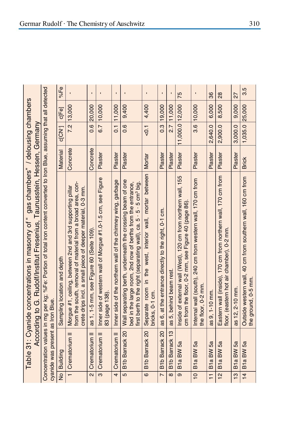
High delousing residues aren’t confined to a thin surface stain. Rudolf’s Table 31 reports R9 at 11,000 mg CN/kg in the 0–2 mm layer, R17 at 13,500 in the 4–10 mm layer, and R20 at 7,850 in the 0–3 mm layer. Their total iron contents were 12,000, 15,000, and 11,000 mg/kg. An explanation must allow substantial cyanide to form and remain, including below the immediate surface. Those total-iron measurements constrain the available inventory, but don’t measure how fast reactive iron reached the reaction sites. Read both pages of the sample table.
The later experiments also preserve positive evidence. Some contaminated soils retained large amounts of iron cyanide, and one loess experiment showed little release after air was restored. Another study recovered the added cyanide across its final soil and aqueous measurements. The recovered 1927 method produced very different results from wall-paint scrapings after dry heating and after acid treatment. These observations constrain loss and assay assumptions. They don’t select a unique HCN-to-pigment yield for the historical walls. The full dossier gives the results and original pages.
A useful bound doesn’t always require complete chemical identification. For a specific assay without positive interference, on a common cyanide-mass basis and with all inputs counted:
The first inequality allows a positive assay of only part of the cyanide to establish a lower bound when the stated specificity and interference conditions hold. It doesn’t settle a disputed interference objection merely by being written as an inequality. The second follows from conservation. Neither inequality by itself gives the proportion of the original dose retained in a sampled wall.
A measured layer can also establish a partial inventory. If its representative concentration is C mg CN/kg, its dry density is ρ kg/m³, and its thickness is d meters, it contains Cρd mg CN/m². Nonnegative cyanide outside that layer makes this a lower bound on the full profile, even for a layer below the surface. No historical wall density is assumed here. Different sampling depths can’t be treated as interchangeable concentrations or made into a measured depth profile by scaling only with total iron.
These bounds show what a better historical comparison can use now. A jointly supported example or a defensible relative bound could answer Rudolf’s exclusion. It wouldn’t require a complete census of every reaction or a unique history for every wall. The numerical example above remains conditional until its material and reaction assumptions are supported together.
Other capture laws and the earlier proportional calculation
The earlier proportional example gives 402 mg/kg for 400 thirty-minute chamber exposures and 2,768 to 2,931 mg/kg for 270 daily six-hour delousing exposures. Its chamber result is about 60 times the initial R3 reading. It doesn't explain the observed gap and isn't used as the main positive result.
For that law, retained cyanide scales directly with integrated exposure, the gas concentration multiplied by time. Once mobile cyanide has drained away, the exchange machinery cancels from the comparison. For nonlinear capture, the time history matters.
| Capture law | 14.4 min | 30 min | 72 min | R12 |
|---|---|---|---|---|
| Proportional | 193 | 402 | 965 | 2,768 |
| Power 1.5 | 54 | 148 | 477 | 2,157 |
| Square law | 11 | 45 | 220 | 1,728 |
The corresponding R13 values are 2,931, 2,284, and 1,830. These earlier nonlinear scenarios use a mobile capacity of 546 mg/kg. The opening example uses 500 mg/kg, a power of 2.10733, and 400 delousing treatments, so it isn't the same scenario with a new label.
The full grid retains the contrary results. With capacity fixed at 500 mg/kg, the aqueous analogue powers give about 8 to 552 mg/kg for 400 short exposures. The near-quadratic example rises to about 192 mg/kg when its chamber rectangle lasts 72 minutes. Other capture and iron-supply assumptions give still higher values. The available experiments don't justify selecting one law as the most likely historical law.
The earlier thirty-minute input was a judgment between the 14.4- and 72-minute branches. Records of removable carriers don't establish a perfect ventilation trace. Rectangles with the same integrated exposure can give different nonlinear retention if their actual concentration histories differ.
Earlier calculation · All earlier numerical results · Complete nonlinear grid
Equations, source pages, and reproducible calculations
The model keeps a cyanide balance
Let M be mobile cyanide, B retained product, E cyanide that has escaped, and Q the equilibrium mobile inventory at the laboratory reference gas concentration. The two exchange contributions are M₁ and M₂, with M = M₁ + M₂. All inventories are in mg CN/kg and time is in hours. The external concentration c is divided by the laboratory reference concentration.
inward supply to contribution i = Q wᵢ c / τᵢ
capture rate r = Q a (M/Q)ⁿ
dMᵢ/dt = Q wᵢ c / τᵢ − Mᵢ/τᵢ − (Mᵢ/M) r
dB/dt = r dE/dt = Σ Mᵢ/τᵢ
M + B + E = cumulative inward supply
Capture is zero when no mobile cyanide remains or the finite iron capacity has been reached. For this example, a = 0.1669961925 h⁻¹, fitted to the laboratory endpoint. The iron reference is 10,000 mg Fe/kg; the ideal Prussian-blue stoichiometry gives a maximum of 11,980.20 mg CN/kg. The corrected exchange weights are 0.18658 and 0.81342, obtained by allowing for the source specimens' 24-hour loading before their release curve was measured. The gas boundary is prescribed. A full wall reconstruction would also need room gas inventory, area, sample thickness, and transport through depth.
Scaling M, B, E, Q, and total capacity together by 0.85 or 0.90 preserves these equations exactly, even with nonlinear capture. Thus the output scaling is mathematically valid under that stated common-material assumption. Whether different historical plasters satisfy it is a separate physical question.
Original conserving model · Calibration results · Schedule and scaling calculations · New numerical results
Todd's experiment measured dissolved ferrocyanide
Todd, Wogan, and Catling, Favorable Environments for the Formation of Ferrocyanide, a Potentially Critical Reagent for Origins of Life, ACS Earth and Space Chemistry 8 (2024), 221–229, equation 4 and Table 1 on page 224. The printed pH 6 power is 2.02 ± 0.09. The model's 2.10733 is the project's separate fit to the published raw measurements, near the upper end of the printed interval. Under the model's calibration, that end gives a lower chamber result. The printed rate constants aren't used. Table 1 gives an order in dissolved iron of −0.104 ± 0.181 at pH 6. That result doesn't establish the model's separate assumption that wall capacity and capture throughput scale with total iron.
Published paper · Raw-data fit · Fitted powers
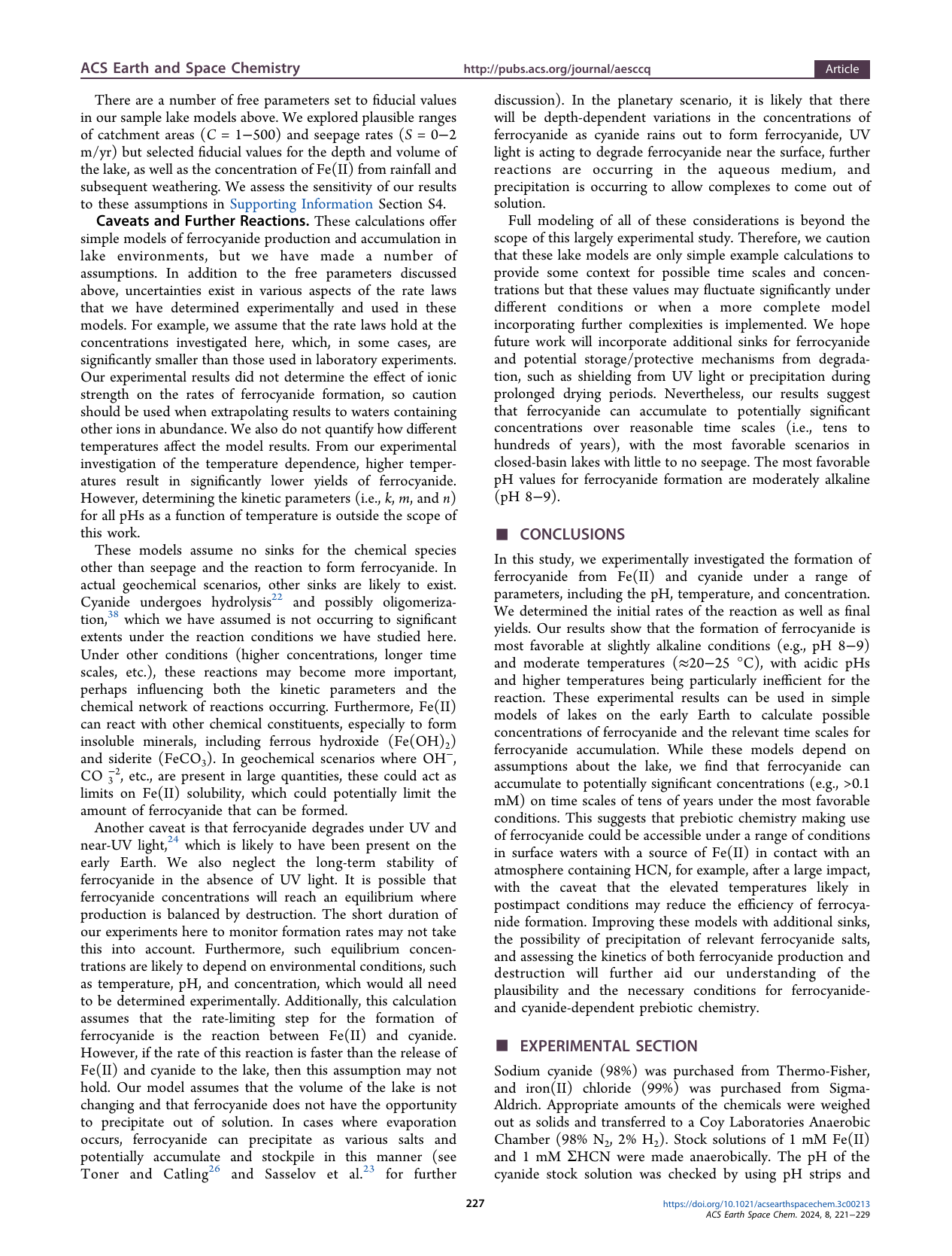
Page 227 states that ionic-strength effects weren't measured, a full temperature-and-pH rate model wasn't determined, other reactions can consume available iron, and reagent delivery can be slower than ferrocyanide formation. The study doesn't measure a masonry capture law or long-term retained pigment.
The mobile-capacity estimate assumes wall water
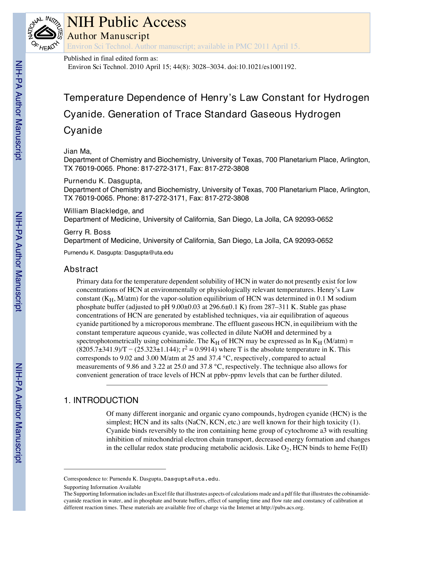
Ma and colleagues, Temperature Dependence of Henry's Law Constant for Hydrogen Cyanide, Environmental Science & Technology 44 (2010), 3028–3034, give ln K = 8205.7/T − 25.323, with T in kelvin and K in mol/L/atm. At 11°C, K is about 35. Multiplying by the 0.02-atmosphere reference gas, 0.03 liters of assumed water per kilogram, and the mass of cyanide groups gives about 546 mg CN/kg.
The experiment covered 287 to 311 K. Its trace-gas conditions were far below 2% HCN. The estimate doesn't add a high-pH ionization multiplier, and doesn't establish the historical pore-water volume. Temperature and water-content calculations.
Rudolf's sample and laboratory tables
The Chemistry of Auschwitz (2020), Table 31, pages 310–311, reports R3, R12, R13, and the laboratory specimens. Pages 327–328 describe the laboratory conditions. R3's sampling depth differs from R12 and R13, and R27 and R28 differ in composition and added water.
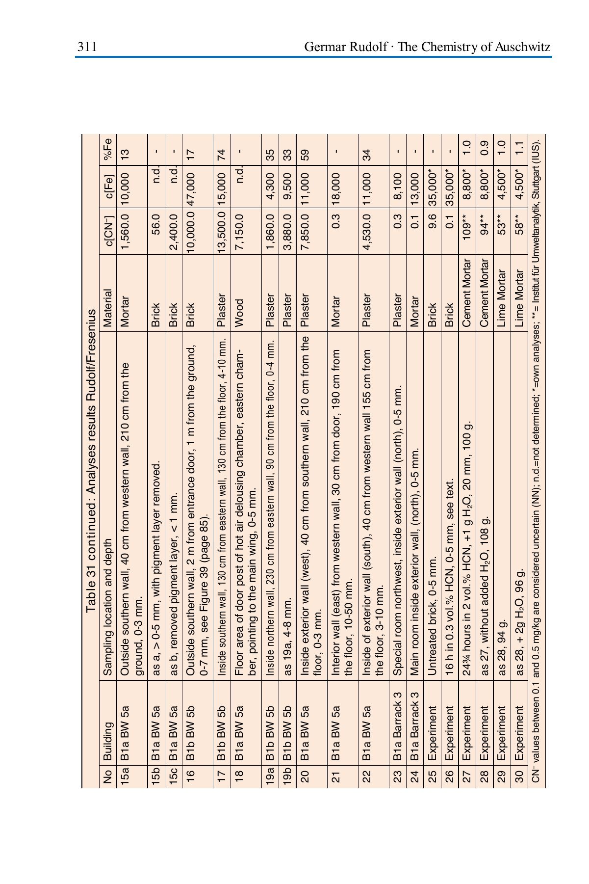
Laboratory conditions, page 327 · Exposure, storage, and specimen differences, page 328 · Release curve, page 225 · Rudolf's residue formula, page 358
Sources on formation and persistence
Meeussen's 1992 thesis contains the equilibrium tables discussed above. Meeussen and colleagues, Solubility of Cyanide in Contaminated Soils (1994), discusses the persistence of Prussian blue despite predicted dissolution. Ware's study of cyanotype conservation (2003) discusses alkaline breakdown. Kamat, Lubelli, and Schlangen, Leaching behaviour of a crystallisation inhibitor in mortars (2023), reports the mortar leaching experiment. These are the complete held publications; the links in the formation section also open the specific reproduced pages.
Blue staining, washing, and CO₂
Rudolf's mortar specimens retained cyanide without visible blue staining. He also accepts Zyklon B use without blue staining at Dachau and Buchenwald and proposes coating and dry, heated air as explanations. These examples make material conditions relevant. They don't independently calculate the low Auschwitz total-cyanide values. The full experiments and comparisons.
The Untergriesbach accounts disagree about colors and reactions. The technical paper identifies calcium cyanide and proposes dark HCN-polymer products; it doesn't identify Prussian blue. That absence of identification isn't proof the pigment was absent. The church and the cited paper.
The separate washing test measured loss from small plaster specimens with a method that excluded Prussian blue. Added CO₂ changed experimental results in both directions across materials. Neither supplies a universal percentage to subtract from a historical wall's total residue. The calculation above uses neither as a numerical loss factor. Washing, weathering, and surviving residues.
Rudolf misrepresents the roof-opening study
In Lectures on the Holocaust, p. 249, Rudolf says Keren and colleagues admitted that none of the openings were made during construction. Their paper expressly argues that Hole 4 was cast during construction in January 1943. That error doesn't settle the chemistry, but it removes the supposed concession he uses to dismiss their findings. Read the comparison with both complete page scans.